pD#l8&K*i+ie4: The Predictability of Faux Randomness Through a Dice Case Study

Abstract

The number that a truly fair die gives off is random and has an equally likely chance to produce any other number. However, the sum of any n number of dice (where n is greater than one) has its frequency be that of the binomial distribution wherein the curve looks more ideal as n gets larger. The sum of two dice that is most frequent is seven. However, just because a single instance of an event is random, it does not imply that there exists no pattern when a compilation of many individual cases is taken. Furthermore, I claim that instances such as the rolling of dice are indeed predictable if one were to know every single initial condition before the event, thus randomness in the macro level is a product of our ignorance and not true randomness. There exists a hard-deterministic result to every supposedly random macro instance.

Introduction

The number that a single fair die produces when it is rolled is, in most cases, random. Similarly, the sum of two dice when they are rolled is unpredictable in a single instance. However, if a compilation of the single instances is made, it becomes evident that dice are more likely than not to produce a sum of seven than any other number. This is because there are more combinations of the dice that make seven than any other number. Let the first die be denoted by the letter ‘D’ and the second die by the letter ‘E’ and the number that follows the die be the number the die rolls. For instance, D4 means that the first die rolled 4 and E2 means the second die rolled 2.

Table 1: The sum of two dice

Notice the diagonal symmetry of the numbers. Out of the 36 different combinations, the most frequent combination is 7 which has a potential combination for each given number, as all numbers can sum to make 7 but not all numbers can sum to make 12 (if a die rolls 2, regardless of the other die the sum cannot be 12).  The sum of 7 is six times more likely to occur than the sum of either 2 or 12. Thus, although a single instance cannot be predicted, the sum of dice roll that is most ubiquitous is 7.

Materials and Procedure

The materials used for this experiment were as follows: 2 six-sided dice. The procedure is as follows:

1) Roll two dice simultaneously and record their individual results and then their sum.

2) Repeat 99 more times.

The author recommends using different colored dice for faster recording of the results, since it is easier to distinguish two idiosyncratic dice than two similar dice. However, the choice of the color of the dice does not have an effect on the results of the experiment.

Results

Since we know that the most likely sum is 7 we expected that to be displayed in the graph. However, since the sample size of 100 trials is not large enough, a skewed result was produced. The expected graph was intended to look like the negative absolute value of x (if a line was made that passes through the center of each of the bars):
(See Appendix Figure 2 for graph of equation 1)

Equation 1:     

(See Appendix Figure 2 for graph of equation 1)

 

Instead the bar graph (on page 4) that was ascertained looked quite different, and if a line were to be drawn through the middle of each bar, it would not look like equation 1 at all. The expected result is Figure 3 in Appendix, where a large sample size is acquired through simulation.

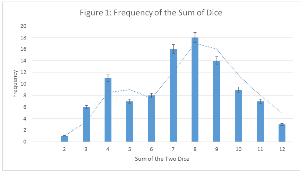
The trend line on this graph is quite different from what was expected. For data of this graph, refer to table 2 in the Appendix.

Analysis of Results

The result was not that which was expected due to the relatively small sample size. A much larger sample size is simulated, and its graph can be found in the Appendix under the title Figure 3 with the trendline of equation 1 plotted onto the graph. The sample size, or the number of rolls is 23,171. If the graph of only one die’s rolls were plotted it would have a horizontal trendline with gradient zero because each side is as statistically likely as other. If enough samples were taken, the frequency of each of the bars would be the same but this can only happen when the number of rolls is divisible by six, or else the graph would not have gradient zero, meaning the trendline would not be flat.

Jonathan D. Baker (2013) argued in his article “Rolling the Dice,” that if we were to jump up to 3 dice rolls, we would see that the trendline would be a bell curve (Figure 4) and if we have 6 consecutive dice rolls then it looks like the binomial distribution (Figure 5). The more and more dice we can simultaneously roll, the closer it the trendline would look like to the ideal binomial distribution. Similarly, this experiment can be statistically interpreted as starting off with a straight line (1 die) and for each additional die added, the graph takes more and more points in between an initial value at x= 0 and y =0 to some arbitrary x where y = 0. Meaning the greater the number of dice, the smaller the interval in the plotting of the function of the binomial distribution and the more accurate the graph becomes. Thus, my conclusion on the properties of the graphs of the frequency of dice rolls is like that of Baker’s, which is that randomness has a predictable frequency and an overall pattern for an adequate amount of sample size.

Conclusion

So far, our analysis and thinking has been in an applied and general sense. But now let us switch our perspective from a statistical and mathematical analysis of the experiment to a more meta-mathematical or metaphysical analysis so we can better reflect on the results rather than be superficial in our analysis. Although this experiment was done to illustrate probability, this was not truly random, meaning being unpredictable and containing no recognizable patterns. Although the dice roll was, practically, unpredictable, it did however, contain a clear recognizable pattern. It is however true that if we were aware of every single parameter of the environment and of our force and torque which launched the dice and the friction of the table onto which the dice was launched and the dimensions of each side of the die (since there are imperfections when manufacturing the die, it is not perfectly cubical and has smooth edges with a different curvature for every edge), then we could calculate the exact face that the die would land on. Probability is thus simply a crutch for our ignorance, it is not that it is literally impossible to predict what might happen given the circumstances, merely that it is extremely hard to figure out. Thus, this experiment does not gauge randomness successfully. But this leads us to question what is random?

The infinite monkey theorem states that given enough time (limit as time extends to infinity) and given enough random cycles (monkeys typing on a typewriter) it is possible for the monkeys, through inputting and concatenating random strings in random locations, to produce the entire works of Shakespeare. Monkeys on a typewriter surely are random but in a given time frame, if one has knowledge of Shakespeare, then the entire work that the monkeys produce randomly and with no conceivable pattern, suddenly has a pattern to it. This is what I mean by faux patterns emerging from real randomness. Consider a quantum die which cannot be (by laws of physics) have its number after it is rolled be predicted until after it has been rolled. Now consider that the die has only one number in all six of its sides, and that one number is 4. Now although the die is entirely random, it still produces a clear and predictable pattern. Thus, it seems to me that our definition of what it means to be random has been corrupted to the point where we cannot discern what is truly random and what is only given the title of random for convenience and for ignorance’s sake. Randomness is hard to identify, it is easier for us to know or claim that something is not random (and be likely right for there is still the threat of false positivity from real randomness) than it is for us to say that something truly is random.

Works Cited

Baker, J. D. (2013). Rolling the Dice. The Mathematics Teacher, 106(7), 551-556. doi:10.5951/mathteacher.106.7.0551, https://www-jstor-org.ccny-proxy1.libr.ccny.cuny.edu/stable/pdf/10.5951/mathteacher.106.7.0551.pdf?refreqid=excelsior%3A8c528774d33d2795516dfc7c2324f2aa, Date Accessed: 3 March 2019

Desmos graph. (n.d.). Retrieved from https://www.desmos.com/calculator

Elmo, Gum, Heather, Holly, Misletoe, and Rowan,Notes Towards the Complete Works of Shakespeare, Web Archive. (n.d) Retrieved from https://web.archive.org/web/20130120215600/http://www.vivaria.net/experiments/notes/publication/NOTES_EN.pdf , Date Accessed: 21 March 2019

Math Forum. (n.d) Retrieved from (n.d.). Retrieved from http://mathforum.org/library/drmath/view/56688.html , Date Accessed: 21 March 2019

Statistics of rolling dice. (n.d.). Retrieved from https://academo.org/demos/dice-roll-statistics/, Date Accessed: 21 March 2019

Appendix

Figure 2: Graph of equation 1 which is -|x| or the negative of the absolute value of x 

This graph of figure 2 was plotted in Desmos, refer to works cited.

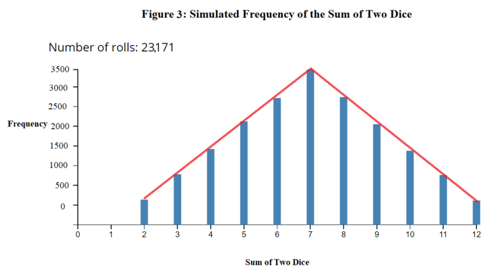
Figure 3-5 are simulated through the help of Academo. Figure 3 was the expected result of experiment and the trend line is equation 1 as expected.

Figure 4 is the sum of three dice which looks like a bell curve or a smoother modulation of equation 1.

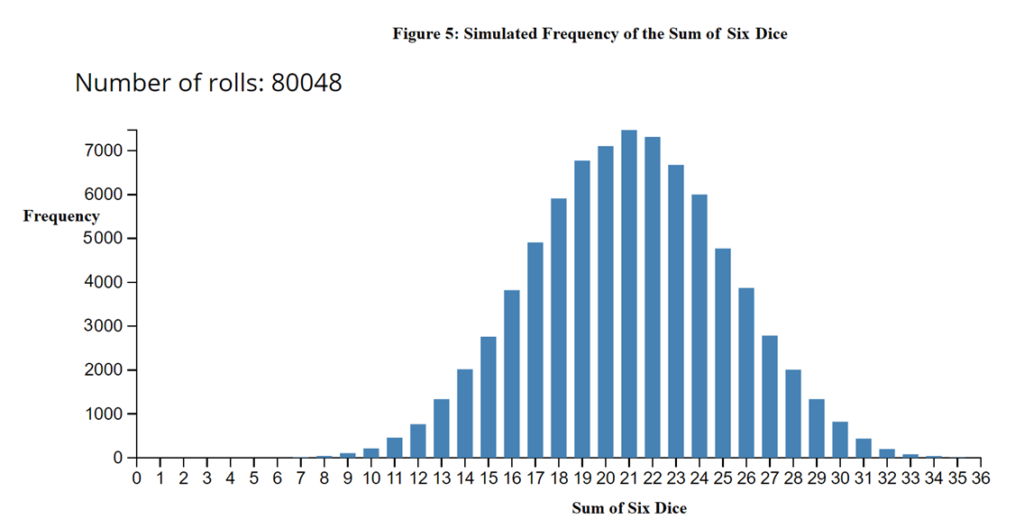
Figure 5 resembles the binomial distribution most accurately as it has the most amount of consecutive dice rolls.

Table 2: Sum of Two Dice Rolls (Empirical Data)

Trial #	Die 1 (D)	Die 2 (E)	Sum of the two dice
1	5	4	9
2	2	2	4
3	6	4	10
4	3	2	5
5	5	3	8
6	3	1	4
7	3	2	5
8	5	2	7
9	4	1	5
10	4	4	8
11	3	1	4
12	6	3	9
13	1	3	4
14	3	2	5
15	6	3	9
16	6	5	11
17	4	4	8
18	2	2	4
19	2	1	3
20	3	4	7
21	6	2	8
22	6	1	7
23	5	3	8
24	3	1	4
25	6	1	7
26	5	4	9
27	6	3	9
28	2	1	3
29	4	4	8
30	5	4	9
31	5	3	8
32	6	4	10
33	6	2	8
34	6	5	11
35	5	1	6
36	6	4	10
37	2	2	4
38	4	3	7
39	3	1	4
40	5	5	10
41	3	1	4
42	6	1	7
43	1	6	7
44	6	3	9
45	3	3	6
46	6	4	10
47	2	1	3
48	4	4	8
49	6	2	8
50	5	1	6
51	5	3	8
52	6	2	8
53	3	3	6
54	6	4	10
55	4	4	8
56	6	1	7
57	2	1	3
58	6	6	12
59	2	5	7
60	6	6	12
61	2	5	7
62	5	2	7
63	6	5	11
64	5	2	7
65	6	6	12
66	3	5	8
67	5	6	11
68	3	6	9
69	5	4	9
70	5	2	7
71	4	6	10
72	5	2	7
73	5	5	10
74	2	4	6
75	6	5	11
76	3	5	8
77	5	1	6
78	1	4	5
79	6	3	9
80	3	5	8
81	2	2	4
82	5	3	8
83	6	5	11
84	2	1	3
85	1	5	6
86	6	3	9
87	3	2	5
88	2	2	4
89	1	6	7
90	3	3	6
91	5	4	9
92	2	1	3
93	1	1	2
94	5	6	11
95	2	5	7
96	4	5	9
97	6	4	10
98	6	2	8
99	5	4	9
100	2	3	5